Back to blog

October 16, 2024

The Problems with p-values

Why Frequentist Significance Testing Falls Short

Taewoon Kim statisticsp-valuesdata sciencefrequentist vs bayesianstatistical significancehypothesis testing

Statistical significance testing, specifically the use of p-values, has been the cornerstone of hypothesis testing for decades. However, this frequentist approach has critical flaws that can lead to misleading interpretations and false confidence in research results. In this post, we will break down why p-values often fall short and discuss how Bayesian methods can offer a clearer and more informative interpretation.

Understanding p-Values: A Quick Recap

The p-value is defined as the probability of observing results at least as extreme as the actual data, assuming the null hypothesis is true:

$p = P(\text{data} \mid H_0)$

Where:

• $p$ is the p-value,
• $H_0$ is the null hypothesis.

If the p-value is less than the predefined significance level (e.g., $\alpha = 0.05$), the result is labeled “statistically significant.” However, this interpretation has led to common misunderstandings.

A Simple Example: The Binomial Test

Let’s take an example where we flip a coin that is very close to fair, with a true probability of heads of 0.501. While this is practically a fair coin, let’s see how p-values behave as we flip it more and more times.

We flip the coin several times: $N = 100$, $N = 1000$, $N = 10,000$, and finally $N = 1,000,000$. After each set of flips, we count the number of heads and calculate the p-value to test whether the coin is significantly different from a fair coin (i.e., $\theta = 0.5$).

Calculating p-Values Using the Gaussian Approximation

For large $N$, the binomial distribution can be approximated by a Gaussian (normal) distribution due to the Central Limit Theorem. This approximation simplifies the calculation of p-values. Here’s how we do it:

1. Define the Parameters:

   • Null Hypothesis: $H_0: \theta = 0.5$
   • Observed Heads: $x$
   • Number of Trials: $N$

2. Calculate the Mean and Standard Deviation:

   Under the null hypothesis, the mean ($\mu$) and standard deviation ($\sigma$) of the binomial distribution are:

   $\mu = N \cdot \theta = N \cdot 0.5$

3. Compute the z-Score:

   The z-score measures how many standard deviations the observed value is from the mean:

4. Determine the p-Value:

   The p-value is the probability of observing a value as extreme as, or more extreme than, the observed value under the null hypothesis. For a two-tailed test:

   $p\text{-value} = 2 \cdot \left(1 - \Phi\left(|z|\right)\right)$

   Where $\Phi$ is the cumulative distribution function (CDF) of the standard normal distribution.

5. Example Calculation:

   Let’s calculate the p-value for $N = 1,000,000$ and $x = 501,000$ heads.

   • Mean: $\mu = 0.5 \times 1,000,000 = 500,000$
   • Standard Deviation: $\sigma = \frac{\sqrt{1,000,000}}{2} = \frac{1000}{2} = 500$
   • z-Score: $z = \frac{501,000 - 500,000}{500} = \frac{1,000}{500} = 2$
   • p-Value: $p\text{-value} = 2 \cdot \left(1 - \Phi(2)\right)$. Using standard normal tables or a calculator, $\Phi(2) \approx 0.9772$. Therefore, $p\text{-value} = 2 \cdot (1 - 0.9772) = 2 \cdot 0.0228 = 0.0456$.

   This p-value is approximately 0.046, which is below the “arbitrary” $\alpha = 0.05$ threshold, leading to a “statistically significant” result.

Here are the results for all the sample sizes:

• For $N = 100$, we observed 51 heads and the p-value was 0.920.
• For $N = 1,000$, we observed 501 heads and the p-value was 0.975.
• For $N = 10,000$, we observed 5010 heads and the p-value was 0.849.
• For $N = 1,000,000$, we observed 501,000 heads and the p-value dropped to 0.046.

The p-Value Problem: It’s Not What You Think

Notice what happened here: as we flipped the coin more times, the p-value gradually decreased. By the time we flipped the coin 1,000,000 times, the p-value dropped below the arbitrary threshold of $\alpha = 0.05$. According to the frequentist approach, this result is “statistically significant,” and one might conclude that the coin is not fair. But really? Are we seriously going to argue that a coin with a 0.501 probability of landing heads is significantly different from a fair coin in any meaningful sense?

This result highlights two fundamental problems:

1. Arbitrary Threshold: The $\alpha = 0.05$ threshold is completely arbitrary. We could easily make $p = 0.046$ insignificant by choosing a slightly stricter $\alpha = 0.01$. There’s no solid reason why $0.05$ should be the magic cutoff.

2. p-Value Decreases with More Data: As we increase the sample size, the p-value decreases—even though the coin remains practically fair. This means that for large datasets, trivial differences can become “statistically significant” even when they are meaningless in the real world.

A Bayesian Approach: Learning from the Data

Now, let’s see how the Bayesian approach can provide a better understanding of the coin’s fairness. Instead of calculating a p-value and making binary decisions, Bayesian methods allow us to update our beliefs about the probability of heads as we observe more data.

Calculating $\theta$ Using Bayesian Inference

In Bayesian inference, we aim to update our belief about the probability of heads, denoted by $\theta$, using observed data. This is done through a process known as posterior updating, where we update our initial belief (the prior distribution) after observing new data (the likelihood).

Bayesian Updating Formula

Mathematically, we use Bayes’ Theorem to calculate the posterior distribution of $\theta$ after observing a series of coin flips:

Where:

• $P(\theta \mid \text{data})$ is the posterior probability distribution for $\theta$, the probability of heads after observing data.
• $P(\text{data} \mid \theta)$ is the likelihood of observing the number of heads given $\theta$.
• $P(\theta)$ is the prior probability distribution of $\theta$, our belief before seeing the data.
• $P(\text{data})$ is the marginal likelihood of the data, a normalizing constant.

Beta Distribution as a Prior

For a Bernoulli process like coin flips, we typically use a Beta distribution as the prior for $\theta$. After observing the data, the posterior distribution of $\theta$ also follows a Beta distribution, making it easy to update.

Let’s say we start with a uniform prior, $\text{Beta}(1, 1)$, which reflects an initial belief that any $\theta$ between 0 and 1 is equally likely. After observing $x$ heads out of $N$ flips, we update the parameters of the Beta distribution:

$\text{Beta}(\alpha_{\text{posterior}}, \beta_{\text{posterior}})$

Where:

• $\alpha_{\text{posterior}} = \alpha_{\text{prior}} + \text{heads observed}$
• $\beta_{\text{posterior}} = \beta_{\text{prior}} + \text{tails observed}$

Example: Bayesian Updating in Action

For example, after observing $N_{\text{heads}}$ heads in $N_{\text{flips}}$ flips, we update our Beta prior as follows:

• Prior: $\text{Beta}(1, 1)$
• Observed heads: $N_{\text{heads}}$
• Observed tails: $N_{\text{tails}}$ = $N_{\text{flips}}$ - $N_{\text{heads}}$

The posterior distribution becomes:

$\text{Beta}(1 + N_{\text{heads}}, 1 + N_{\text{tails}})$

This updated Beta distribution gives us a refined estimate of the probability of heads, $\theta$, while also reflecting the uncertainty around that estimate. As we gather more data, the posterior distribution will become narrower, indicating greater certainty in our estimate of $\theta$.

Visualizing the Posterior Distributions

Let’s now visualize how the Bayesian posterior distribution changes as we increase the number of coin flips, similar to the frequentist example. Instead of focusing on a single point estimate like in the frequentist method, the Bayesian approach updates the full distribution of $\theta$, capturing both the estimate and our uncertainty.

The following figure shows how the posterior distribution becomes more concentrated as the number of flips increases:

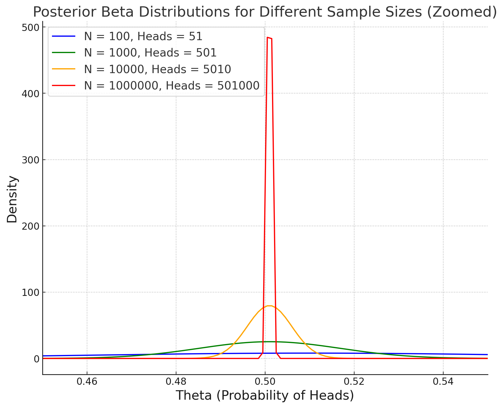
In this plot, we can see that:

• For $N = 100$, the posterior distribution is relatively wide, indicating a fair amount of uncertainty around $\theta$.
• For $N = 1,000$, the distribution is narrower, meaning we are more certain about $\theta$.
• For $N = 10,000$, the distribution becomes even more concentrated.
• For $N = 1,000,000$, the posterior distribution is very sharply centered around $\theta = 0.501$, indicating that we are highly certain about the true probability of heads.

As we collect more data, the posterior distribution approaches a Dirac delta function centered around the true value of $\theta = 0.501$. This illustrates how Bayesian inference provides a clearer picture of our growing certainty as the sample size increases. Unlike p-values, which can be misleading with large sample sizes, the Bayesian approach shows that we are converging to the true value of $\theta$ with increasing certainty.

Key Insight: Certainty Increases with More Data

The crucial difference between the frequentist and Bayesian approaches is this: while p-values tend to drop with increasing sample sizes—sometimes leading to statistically significant results even for trivial effects—the Bayesian approach directly quantifies our certainty about the true value of $\theta$. As the number of observations increases, the posterior distribution narrows, signaling that we are more confident in our estimate of $\theta$.

So, after all this analysis, we might conclude that $\theta$ is very close to 0.501. But wait—does this mean the coin is truly fair? Should we say this is a fair coin then? The Bayesian approach allows us to answer this with further analysis, specifically through Bayesian Hypothesis Testing, which directly compares hypotheses. However, that is a topic for a future post.

Conclusion: Moving Beyond p-Values

The p-value-based frequentist approach to statistical significance is not only limited but can also be misleading. In our coin flip example, increasing the number of flips caused the p-value to drop below the arbitrary threshold of $\alpha = 0.05$, leading to the incorrect conclusion that the coin is biased. In contrast, the Bayesian approach allows us to continuously update our understanding of the coin’s fairness based on the observed data, and as we gather more flips, we get closer to the true probability of heads.

Bayesian methods offer a richer and more nuanced interpretation of data, free from the arbitrary thresholds and misleading binary decisions that p-values impose. Instead of focusing on binary outcomes (significant vs. not significant), the Bayesian approach allows us to quantify our uncertainty and increase our confidence as more data is gathered. It’s time to move beyond p-values and embrace methods that allow us to learn from data in a more flexible and informative way.